Introduction to the Lambda Calculus, Part 1

This is part 1 of a two-part reading on the lambda calculus. In this reading, I introduce the lambda calculus, its origins and purpose, and discuss its syntax. In the second reading, I will discuss its semantics.

Introduction

The lambda calculus is a model of computation. It was invented in the 1930’s by the mathematician Alonzo Church, who like his contemporary, Alan Turing, was interested in understanding what computers were capable of doing in principle.

For me, there are three really remarkable things about the lambda calculus.

Although this fact has never been proven, it is widely believed that the lambda calculus is capable of expressing any computation.
It was invented before any computers actually existed in the real world.
It is really, really simple.

The lambda calculus is equivalent in expressive power to that other famous model for computation, the Turing machine. Unlike the Turing machine, though, the lambda calculus has an elegance to it that the Turing machine lacks. For starters, with some effort, you can understand a “program” written in the lambda calculus. It is incredibly difficult to understand any kind of “program” written for a Turing machine, because a Turing machine closely corresponds to a mechanical computer. The lambda calculus, on the other hand, is essentially the language of functions.

As a result, the lambda calculus serves as the theoretical foundation for many real programming languages, most notably LISP. More modern languages, like ML and Haskell, are also deeply influenced by the lambda calculus. Many ideas that came from the lambda calculus, like “anonymous functions,” have found their way into bread-and-butter languages like Javascript, Java, C#, and even C++. When we talk about “functional programming,” at its core, what we’re talking about is the lambda calculus.

The lambda calculus as a programming language

The lambda calculus can be thought of as a kind of minimal, universal programming language. What do I mean by “minimal”? I mean that it is small and that its features are essential in some way. By “universal” I mean that it is capable of expressing all computable functions. While it is probably not the most minimal programming language (in fact, the Intel mov instruction all by itself has the same expressive power), it is the most useful minimal language that I know of. We will talk about what a computable function is later; for now, understand it to mean that an ideal computer should be capable of computing it.

Formal definitions

Since I claim that the lambda calculus is like a programming language, we ought to be able to examine it formally like a programming language. Most formal specifications of a language come in two pieces: (1) syntax and (2) semantics.

Syntax is the “surface appearance” of a programming language. For example, the following snippets are from Java and F#, respectively:

Java:

int sum(List<Integer> lst) {
  int accumulator = 0;
  for (Integer i: lst) {
    accumulator += i;
  }
  return accumulator;
}

F#:

let sum xs
	let mutable accumulator = 0
	for x in xs do
		accumulator <- accumulator + x
	accumulator

These two languages have different syntax, so they look different; they use different words. But both sum functions written here convey exactly the same meaning. Therefore, the two functions have the same semantics.

Syntax of the lambda calculus

So let’s start with the appearance of the lambda calculus. What does it look like?

Here’s one of the simplest functions you can write in the lambda calculus: the identity function.

λx.x

You might have seen this in algebra before. It looks something like:

f(x) = x

Or maybe Java?

T identity<T>(T t) {
	return t;
}

The lambda calculus version expresses exactly the same concept as the algebraic and Java versions.

Actually, the lambda version is more concise: In the algebra version and the Java version, functions are named. In the algebraic expression above, the function is named f. In the Java version is it called identity. In the lambda calculus, functions do not have names associated with them. They are all anonymous. Why? Because Church was looking for a minimal model of computation. As it turns out, function names are not essential.

Backus-Naur form

Syntax is the arrangement of words and phrases to create well-formed sentences in a language. When we say well-formed, what we mostly mean is that we are not just stringing together words arbitrarily, forming nonsense. Instead, there are rules that dictate how words go together. These rules ensure that sentences in our language follow patterns that allow us to extract conventional meanings from them.

The rules that define a syntax are called a grammar. The bootstrapping problem of how exactly one comes up with a language that describes languages dates back to Indian scholars of antiquity. In the 1950’s, John Backus and Peter Naur devised a simple, formal solution. Using their system, one can “generate” all of the valid sentences belonging to a language. That system is now known as Backus-Naur form, or BNF.

Here is the grammar for the lambda calculus:

<expression>  ::= <variable>
               |  <abstraction>
               |  <application>
			  
<variable>    ::= x
<abstraction> ::= λ<variable>.<expression>
<application> ::= <expression><expression>

This grammar is important enough–and simple enough–that I suggest that you memorize it.

BNF has two kinds of grammar constructions: nonterminals and terminals. In the grammar above, nonterminals are written between angle brackets (< and >). Other characters or words are terminals. I will explain what these things mean in a moment.

The ::= means “is defined as” and the | means “alternatively.” So if you read the definition literally, it says:

<expression> is defined as <variable>.

Alternatively, <expression> is defined as <abstraction>.

Alternatively, <expression> is defined as <application>.

<variable> is defined as x.

<abstraction> is defined as λ<variable>.<expression>.

<application> is defined as <expression><expression>.

Each line in the grammar is known as a production rule (or just rule for short), because it produces valid syntax. If you start with the “top level” nonterminal <expression>, and follow the production rules, when you finally have a sentence that contains only terminals, you now have a valid sentence in the grammar. Since our grammar is for the lambda calculus, this means that you have a valid lambda expression (program).

Following a rule is called an expansion. Let’s try a couple expansions and see what kind of sentences we can get.

Example 1:

Start with <expression>.
```
 <expression>
```
Expand it into either <variable>, <abstraction>, or <application>. Let’s choose <variable>.
```
 <variable>
```
If we look at our definition for variable, there is not much choice. It must be expanded into one thing only:
```
x
```

Since no nonterminals remain, we now know that x is a valid lambda calculus program.

Example 2:

Start with <expression>.
```
 <expression>
```
Let’s expand it into <abstraction>.
```
 <abstraction>
```
This also expands into the following.
```
λ<variable>.<expression>
```
As we know, <variable> only expands into one thing, x, but <expression> could be many things.
```
λx.<expression>
```
It should be apparent, at this point, that this process is recursive. Since we don’t have all day, let’s expand <expression> into <variable> and choose x again.
```
λx.x
```

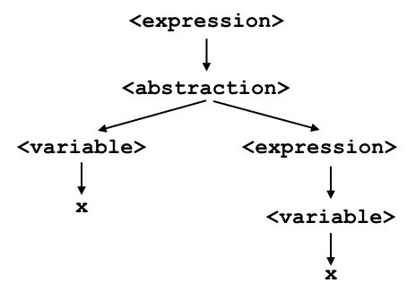
Since no nonterminals remain, we now know that λx.x is a valid lambda calculus program. In fact, it’s the identity function we discussed before.

Parsing

If you think about the kind of sentence generation we did above as a function, at a high level, it would look something like this (pay attention to the parameters and return types):

Sentence generate(Grammar g) {
  // algorithm
}

Parsing is, in some ways, the converse:

bool parse(Sentence s, Grammar g) {
  // algorithm
}

In other words, instead of generating a sentence in a grammar, a parser recognizes whether a sentence belongs to a grammar. If a sentence can be generated from a grammar, parse returns true. If a sentence cannot be generated, parse returns false.

In practice, we often expand the definition of parse a tad so that, if parse would return true, it returns a derivation, otherwise it returns null.

For example, we already know that λx.x parses, but what does its derivation look like?

In programming languages, a derivation has a special name: we call it a syntax tree, because it shows how the parts of a program are related to each other. Understanding how a lambda expression parses will help you understand how you can “compute” things using it.

Precedence and Associativity

A few little details often trip up newcomers to the lambda calculus. These details rely on concepts called precedence and associativity.

Precedence

The dictionary defines “precedence” as the condition of being more important than other things, and this is essentially the same idea when we talk about languages. Precedence in a programming language means that certain operations are evaluated before others. Using algebra again as an example, this should already be familiar to you. For example, you know that the algebraic expression

x + y * z

needs to be evaluated by first multiplying y and z, then finally by adding x to the product. Without the rule that says that multiplication has higher precedence than addition, the above expression would be ambiguous, because it could be parsed in one of two ways:

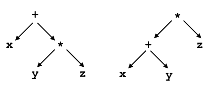
You probably recognize that the parse on the left is the correct one, because it implies that the addition depends on the multiplication, not that the multiplication depends on the addition.

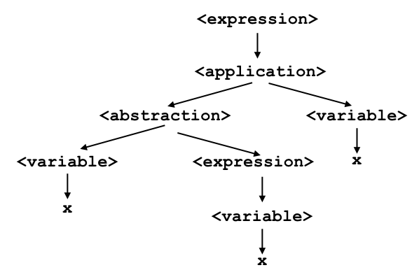
Therefore, precedence is used to remove ambiguity from a language. In the lambda calculus, application has higher precedence than abstraction. This means that if you have an expression like

λx.xx

you should understand it to mean

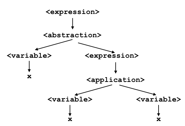
and not

Associativity

Even with precedence, we are occasionally faced with ambiguity. For example, the lambda expression

xxx

Should we think of this expression as (xx)x or x(xx)? Both forms utilize application. We know that application has higher precedence than abstraction, but there’s no abstraction here. Just two different ways to apply the application rule. Associativity solves this problem.

Associativity rules tell us, in cases where the precedence is the same, which parse we should choose.

Application is left-associative. Therefore, we group application expressions to the left ((xx)x) instead of to the right (x(xx)).

We also have the same problem with lambda abstractions. For example,

λx.xλx.x

Should we interpret this expression as λx.(xλx.x) or as (λx.x)(λx.x)? In other words, how much of the sentence is included in the expression that comes after the first period?

Abstraction is right-associative. I like to think of this as meaning that “the period is greedy.” The expression after the period extends as far to the right as makes sense logically. So the correct interpretation is actually λx.(xλx.x).

These rules take a little time to internalize, but after some practice, you will eventually get the hang of them.