Introduction to the Lambda Calculus, Part 2
In our second reading on the lambda calculus, we finish up discussing syntax and move on to the semantics of the language.
Ambiguity
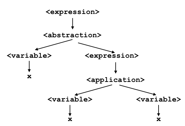
In our last reading, we looked at an expression λx.xx and asked what its parse tree should look like. Is it
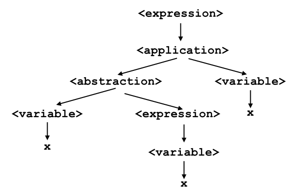
or
?
I told you that, because abstraction is right-associative, the correct interpretation is the first tree.
But what if you wanted to encode the second tree as a lambda program? Without writing your program in separate pieces, such as
a is λx.x
and
b is x
so the whole expression is
ab
then there does not appear to be a way to encode the second tree. Unless you add parentheses to the language.
Parentheses
Parentheses remove ambiguity.
First, let’s introduce a simple axiom into our system:
(<expression>) = <expression>
This axiom says that an expression with parens means the same thing as an expression without them. With this rule, you can feel free to surround an expression with parens, or if the expression is not ambiguous, to remove them.
Second, let’s augment our grammar so that we don’t run into any more ambiguity traps.
<expression>  ::= <variable>
               |  <abstraction>
               |  <application>
               |  <parens>

<variable>    ::= x
<abstraction> ::= λ<variable>.<expression>
<application> ::= <expression><expression>
<parens>      ::= (<expression>)
Now we can avoid the problem with λx.xx. If we write λx.xx, the interpretation, because abstraction is right associative, is:
and if we write (λx.x)x then the interpretation is
Note that it is conventional, among people who use the lambda calculus, to drop parenthesis whenever the interpretation is not ambiguous. Googling for lambda expressions will often turn up scads of examples that omit parens. If you are aware of this fact, many of these examples will be easier to interpret.
Other extensions
Additional variables make the grammar easier to work with.
Here is our new grammar:
<expression>  ::= <variable>
               |  <abstraction>
               |  <application>
               |  <parens>

<variable>    ::= α ∈ { a ... z }
<abstraction> ::= λ<variable>.<expression>
<application> ::= <expression><expression>
<parens>      ::= (<expression>)
where, hopefully, it is clear that α ∈ { a ... z } denotes any letter. E.g., any letter could be x or y, or b, or g, etc.
Finally, to make the lambda calculus more immediately useful, let’s add one more rule, <arithmetic>. Note that this rule is not strictly required, because arithmetic can be encoded using all of the pieces we’ve already talked about. But learning those encodings can be difficult and they are not required to understand the lambda calculus, so we will put them off until later.
An example of arithmetic of the kind we’re talking about might be 1 + 1. To make 1 + 1 a valid <arithmetic> expression, we will write all arithmetic in prefix form. In prefix form,
- The entire expression is enclosed within parentheses.
- The operator is first term written inside the parentheses.
- All subsequent terms written after the operation, but still within the parentheses, are operands.
Formally,
<arithmetic> ::= (<op> <expression> ... <expression>)
For example, 1 + 1 is written as (+ 1 1). Another example is c / z, which is written (/ c z).
What is <op>? A simple formulation might include just +, -, *, and /. I will stick to + and - in this class.
Finally, what is <value>? It is either a number or an <variable>.
<expression>   ::= <value>
                |  <abstraction>
                |  <application>
                |  <parens>
                |  <arithmetic>

<value>        ::= v ∈ ℕ
                |  <variable>
<variable>     ::= α ∈ { a ... z }
<abstraction>  ::= λ<variable>.<expression>
<application>  ::= <expression><expression>
<parens>       ::= (<expression>)
<arithmetic>   ::= (<op> <expression> ... <expression>)
<op>           ::= o ∈ { +, - }
One nice thing about prefix form, which is why we’re using it here, is that the order of operations is very clear. For example, with a little practice, you should have no difficulty computing (+ 3 (* 5 4)). Recall that the equivalent expression in “normal” arithmetic might be written as 3 + 5 * 4, which is ambiguous if you don’t remember your precedence and associativity rules from algebra class.
You can see why I don’t introduce these complications all up front: the grammar is starting to look a little hairy. Still, if you remember that there are essentially three parts to the lambda calculus, variables, abstractions, and applications, you will be fine. To recap, we added:
- Parentheses to remove ambiguity.
- Extra variables.
- Simple arithmetic in prefix form.
Semantics of the Lambda Calculus
Semantics is the study of meaning. In the context of programming languages, what we usually care about is how an expression can be converted into a sequence of mechanical steps that can be performed by a machine.
So how do we interpret the meaning of a lambda expression?
Unfortunately, the word “interpret” is vague. There are two meanings for the word “interpret”:
- To understand.
- To evaluate.
In programming languages, and more generally in computer science, we tend to favor the latter definition of the word “interpret,” i.e., to evaluate. Why? Because evaluation is a mechanistic process. In a well-designed programming language, there is no room for ambiguity. Precision is what sets programming languages apart from natural languages. It is why we can precisely describe programs and run them billions of times without error. But it also means, because they are so different from natural languages, that they are usually quite difficult to learn.
Evaluation via term rewriting
The lambda calculus is an example of a term rewriting system. You’ve seen a term rewriting system before. The system of mathematics you learned in high school–algebra–is a term rewriting system. The big idea behind term rewriting systems is that, by following simple substitution rules, you can “solve” the system. In algebra, we mix term rewriting (substitution) and arithmetic (e.g., 1 + 2) to solve for the value of a variable.
The amazing and surprising fact about the lambda calculus is that term rewriting is sufficient to compute anything. Yes, really, all you need to do is follow a few simple rewriting rules, just like in algebra, and you don’t even need the arithmetical part.
That said, if you intend to compute “interesting” things–the kinds of programs we normally write–the language is hard to work with. Although it is not as primitive as a Turing machine, it’s pretty darned primitive. Alonzo Church’s contribution was to show that the functions we most care about–the ones that are computable in principle–can be written as lambda expressions. This is the reason why I added <arithmetic> to our syntax: without it, doing useful things requires a lot of work, but this one simple extension makes the language useful without sacrificing much of its simplicity.
There are essentially two rewriting rules in the lambda calculus. To understand them, I need to introduce few things first: equivalence and bound/free variables.
Equivalence
In the lambda calculus, we say that two expressions are equivalent when they are lexically identical. In other words, when they have exactly the same string of characters. For example, the expression λx.x and the expression λy.y mean exactly the same thing, but they are not equivalent because they literally have different letters in them. λx.x and λx.x are equivalent, however, because they are exactly the same.
We often talk a little informally about equivalence and you might hear someone say that λx.x and λy.y “are equivalent.” What they mean is that, after rewriting, the two expressions can be made equivalent.
Bound and free variables
Depending on where a variable appears in a lambda expression, it is either bound or free.
What is a bound variable? A bound variable is a variable named in a lambda abstraction. For example, in the expression
λx.<expression>
where <expression> denotes some expression that I don’t care about at the moment, x is the bound variable. How do we know that it is bound? Well, that’s precisely what a lambda abstraction means.
x is a variable, and when x is used inside of <expression>, its value takes on whatever value is passed into the function. To give you an analogy in a language with which you might be more familiar (Python), you can informally think of the bound variable in the above expression to mean almost exactly the same thing as the parameter in the following program:
def foo(x):
	<expression>
except that in the lambda calculus, functions don’t have names (i.e., no foo).
Now it should make sense to you when I say that x is a bound variable. When we call foo, for example, foo(3), we know that wherever we see x in the function body, we should substitute in the value 3. Let’s say we have the Python program:
plus_one(x):
	return x + 1
Then the expression
plus_one(3)
means
3 + 1
Until we actually call the function, x could pretty much be anything; it’s just a parameter. Its value is tied to the calling of the function.
Back to the lambda calculus. In the following expression,
λx.x
both instances of x are bound. How do we know? Because the lambda abstraction tells us that the value of any x within its scope (remember: abstraction is right-associative) is bound to the parameter x.
What about the following expression?
λx.y
The lambda abstraction tells us that x is bound but it says nothing about y. In fact, we can’t really make any assumptions about y. Therefore, we call y a free variable.
To understand a lambda expression, you must always determine whether every variable is bound or free. Be careful! Consider the following expression:
λx.λy.xy
Both x and y are bound. Why? Let’s rewrite using parens. Let’s start with the rightmost lambda. We know, because of right-associativity, that everything to the right of the last period must belong to the rightmost lambda. So,
λx.λy.(xy)
We also know that everything to the right of the leftmost period must belong to the first lambda.
λx.(λy.(xy))
Is the rightmost y bound or free? It is bound because it is within the scope of the λy.___ abstraction. What about the rightmost x? It is also bound, because it is within the scope of the λx.___ abstraction. If you don’t believe me, just look at the outermost parens:
λx.(... x ...)
Here’s a more complicated example with a free variable:
(λx.x)y
Can you spot which one is free?
(ʎ s,ʇᴉ)
One more:
λx.λx.xx
Which variables are bound?
In this case, all the xes you see are bound. However, there are two x variables. Let’s put in some parens to make the expression easier to understand.
λx.(λx.(xx))
So both x values are within the scope of both lambda abstractions. So to which abstraction is x bound? In the lambda calculus, the last abstraction wins. Therefore, it is as if λx.(λx.(xx)) were written
λy.(λx.(xx))
and to give you an intuitive sense of this, this is more or less equivalent to the following (perfectly valid) Python program:
def yfunc(y):
	def xfunc(x):
		return x(x)
	return xfunc
But, of course, without function names. I’ll let you puzzle that for a bit.
Reductions
The rules used to rewrite expressions are called reduction rules.
α Reduction
The first rewriting rule is called alpha reduction. Alpha reduction is a rule introduced to deal with ambiguity surrounding the use of variables. Specifically, alpha reduction relies on the property that, in the lambda calculus, the name of a bound variable does not matter.
Let’s look at a concrete example. Remember the identity function?
def identity(x):
	return x
It returns whatever we give it. Here’s a Python interpreter session:
$ python
Python 2.7.15 (default, Aug 22 2018, 16:36:18)
[GCC 4.2.1 Compatible Apple LLVM 9.1.0 (clang-902.0.39.2)] on darwin
Type "help", "copyright", "credits" or "license" for more information.
>>> def identity(x):
...     return x
...
>>> identity(3)
3
Hopefully no surprises there, right? What if, after we explored the above definition of identity, I asked you what the following function meant:
def identity2(z):
    return z
I suspect that you might be a little annoyed. Why? Because obviously identity1 and identity2 are the same function.
In the lambda calculus, though, remember that we have a strict notion of equivalence. Two expressions are equivalent if and only if they are exactly the same string. So even though identity in the lambda calculus is:
λx.x
and identity2 in the lambda calculus is:
λy.y
and we can sort of squint and see that they’re the same, that’s not enough. We have to prove it.
α Equivalence
The notation [a/b] c means “replace the variable b with variable a in expression c.” To perform alpha reduction, we rely on the following property, which is called “alpha equivalence”:
λx1 .e =α λx2 .[x2 /x1 ] e
where x1 and x2 are variables, e is an expression.
This property says that whenever you have an expression of the form λx1 .e you can replace it with an expression of the form λx2 .[x2 /x1 ] e . The two expressions are “alpha equivalent” (that’s what =α means). Since [x2 /x1 ] is not a valid lambda-calculus expression, you must continue replacement of x1 with x2 wherever you find it in e. You continue doing this until you can proceed no further with substitution.
Here’s a proof that the two expressions are the same.
λx.x                 | given
[y/x] λx.x           | alpha reduce x with y
λy.[y/x] x           | step 1: rename outer x and continue to inner expression
λy.y                 | step 2: rename inner x
Therefore, λx.x =α λy.y.
I mentioned before that sometimes you can “proceed no further with substitution”. Substitution can be “blocked” by nested lambdas. Recall the expression from before:
λx.λx.xx
You might be wondering: is this expression equivalent to λy.λx.yy?
This is a perfect time to do alpha reduction. Let’s replace x with y.
λx.λx.xx             | given
[y/x] λx.λx.xx       | alpha reduce x with y
λy.[y/x] λx.xx       | step 1: rename outer x and continue to inner expression
λy.λx.xx             | done (blocked by λx)
We cannot rename the x inside the inner expression because it is a different x than the outer x. The inner lambda “redefines” x. Therefore λx.λx.xx is not equivalent to λy.λx.yy, at least not using alpha reduction.
When two expressions can be made equivalent using alpha reduction, we call them alpha equivalent.
β Reduction
There is one other kind of reduction called beta reduction. Beta reduction is the beating heart of the lambda calculus because it is, essentially, what it means to call a function. We refer to calling a lambda function application.
The simplest possible example uses the identity function:
λx.x
Let’s “call” this function with a value. Say, y.
(λx.x)y
(Recall that we use parentheses to make this expression unambiguous.)
At a high level. This expression has two parts: left and right. The left side is λx.x. The right side is y. How do we know? The parens tell us.
What is the one grammar rule in the lambda calculus that lets us interpret an expression with a left part and a right part? It’s this rule:
<application> ::= <expression><expression>
Colloquially, we call the left part the function and the right part the argument. Why? Because those two parts work just like the function and argument parts you might see in a conventional programming language.
(λx.x)y
works just like
def identity(x):
	return x

identity(y)
Because we expect to get y back when we call the identity function with y as an argument†.
β Equivalence
Beta reduction is a substitution rule that achieves exactly the same effect. We again use the substitution operation, [a/b] c which means “substitute variable b with expression a in the expression c”, but in the case of beta reduction, substitution eliminates both the function (the lambda abstraction) and its argument.
We rely on the following property, which is called “beta equivalence”:
(λx1 .e) x2 =β [x2 /x1 ] e
where x1 is a variable, and x2 and e are expressions.
This property says that whenever you have an expression of the form (λx1 .e) x2 you can replace it with an expression of the form [x2 /x1 ] e . The two expressions are “beta equivalent” (that’s what =β means). Since [x2 /x1 ] is not a valid lambda-calculus expression, you must continue replacement of x1 with x2 whereever you find it in e. You continue doing this until you can proceed no further with substitution. As with alpha reduction, redefinition of a variable inside a lambda “blocks” substitution.
Example:
(λx.x)y           | given
([y/x] x)         | beta reduce x with y, step 1: eliminate abstraction and argument; continue to inner expression
(y)               | step 2: replace x with y
y                 | eliminate parens (because "<expression> = (<expression>)")
Let’s look at another example.
(λx.xx)z          | given
([z/x] xx)        | beta reduce x with z, step 1: eliminate abstraction and argument; continue to inner expression
(zz)              | step 2: replace x with z
zz                | eliminate parens
In the fourth step, we beta reduce inside the application xx because [z/x] <expression><expression> means [z/x]<expression> [z/x]<expression>.
†The exact Python equivalent to (λx.x)y is actually (lambda x: x)(y). Python will complain that y is not defined if you do not define it somewhere; the lambda calculus is less strict because it doesn’t really care if y is free. Python is an eager language, which essentially means that variables can never be free.
Normal form
When do we stop doing reductions? We stop when there is no beta reduction left to do, and when alpha reduction is just pointless renaming of variables. We say that these expressions are in normal form.
For example, the following expressions are already in normal form:
x
xx
λx.y
xz
However, the following are not:
(λx.x)(λx.x)
(λx.λx.z)y
y(λx.xx)(λx.xx)
Reduction order
In the lambda calculus, the order of reductions does not matter. Any reduction order that terminates will find the normal form, if a normal form exists. Some expressions have no normal form.
The two main reduction strategies are called normal order and applicative order. They differ in an important way:
Normal order: If a normal form exists for expression e, then the normal order reduction will find it.
Applicative order: If a normal form exists for expression e, then the applicative order reduction may find it.
Note the difference. Applicative order may not find the normal form, even if one exists. The reason? Applicative order does not always terminate.
Normal order may also not terminate. However, it only does not terminate in exactly those cases where a normal form does not exist.
You might be wondering why we even care about applicative order. It turns out that this order is equivalent to the order employed by most ordinary programming languages like Java and C! We call this kind of program evaluation eager evaluation. Very few languages utilize the normal order because it is difficult to implement, however there are examples. Haskell, for example, uses the normal order utilizing a form of evaluation we call lazy evaluation.
So what are normal and applicative order reductions?
Normal order
The normal order reduction is the “leftmost” reduction. Here’s an example of a function where you have a choice as to the reduction:
(λx.y)((λa.aa)(λb.bb))
There are two beta reductions available. Let’s label the pieces.
- One beta reduction applies the argument
((λa.aa)(λb.bb))to the function(λx.y). - Another beta reduction applies the argument
(λb.bb)to the function(λa.aa).
To determine the “leftmost reduction”, which of these has the leftmost component? Think of this as asking you: which one has the smallest string index into the original string?
The first beta reduction starts where (λx.y) starts,
(λx.y)((λa.aa)(λb.bb))
^
which is index 0.
The second beta reduction starts where (λa.aa) starts,
(λx.y)((λa.aa)(λb.bb))
       ^
which is index 7.
0 < 7, so the leftmost reduction is the first one.
Always following the leftmost beta reduction, at every step, is the normal order reduction.
Let’s reduce this expression using the normal order:
(λx.y)((λa.aa)(λb.bb))       | given
([((λa.aa)(λb.bb))/x] y)     | β reduce
y                            | substitute & done
Applicative order
The applicative order is to always follow the rightmost beta reduction at every step.
Let’s reduce this expression using the applicative order:
(λx.y)((λa.aa)(λb.bb))       | given
(λx.y)(([(λb.bb)/a] aa))     | β reduce
(λx.y)((λb.bb)(λb.bb))       | substitute & α reduce
(λx.y)((λa.[a/b] bb)(λb.bb)) | sub
(λx.y)((λa.aa)(λb.bb))       | uh-oh... we're back to where we started
...
In this case, the applicative order reduction does not terminate even though we proved that the expression has a normal form when reduced using the normal order.